This post is the first in a series to follow-up on my 2012 GPU Pro 3 article about atmospheric scattering [11]. What I showed there was a full single-scattering solution for a planetary atmosphere running in a pixel shader, dynamic and in real time, without pre-computation or simplifying assumptions. The key to this achievement was a novel and efficient way to evaluate the Chapman function [2], hence the title. In the time since then I have improved on the algorithm and extended it to include aspects of multiple scattering. The latter causes horizontal diffusion (twilight situations) and vertical diffusion (deep atmospheres), and neither can be ignored for a general atmosphere renderer in a space game, for example.
I have written a Shadertoy that reflects the current state of affairs. It’s a mini flight simulator that also features clouds, and other rendering goodies. A WebGL 2 capable browser is needed to run it. Under Windows, the ANGLE/Direct 3D translator may take a long time to compile it (up to a minute is nothing unusual, but it runs fast afterwards). When successfully compiled it should look like this:
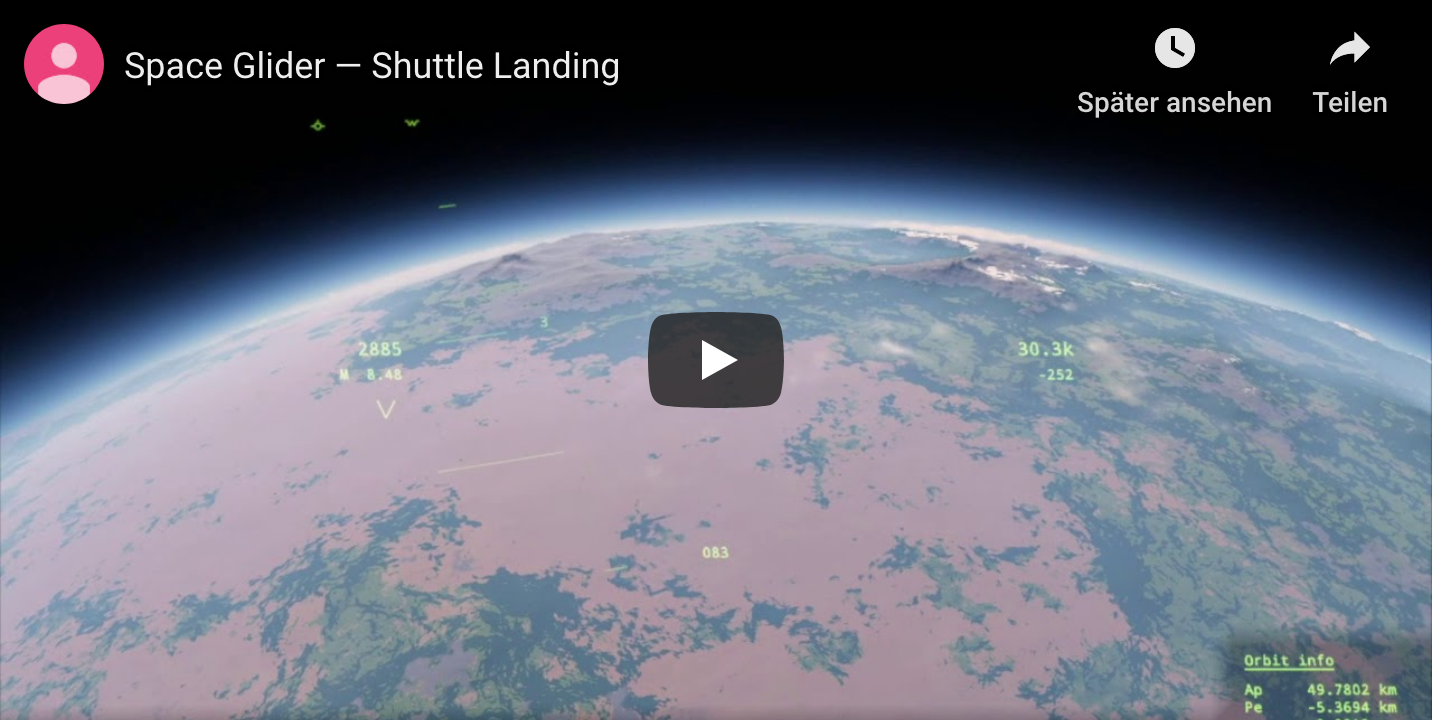
A little background story
The origins of my technique go back to experiments I did privately while hacking on my old Space Glider. Originally this was a demo written for DOS/DJGPP without 3‑D acceleration. It featured a mini solar system with non-photorealistic graphics, in the style of Mercenary and Starglider. Sometime I dusted it off and wanted to make it more real™: larger scale, atmospheric scattering, procedural terrain, HDR, dynamic light adaptation, secondary illumination from celestial bodies, spherical harmonics, real flight dynamics, real orbital mechanics, all that …, you know, a real™ space simulator needs. Naturally, the source didn’t get prettier in the process and the project became an unreleasable mess.
Nevertheless, I came up with a working prototype that had scattering and a procedural terrain. Since it was all calculated on the CPU it had to be super efficient. I devised an analytical approximation to the airmass integral (what later became the Chapman function) so I could reduce the numerical integration from two nested loops to one loop. I made heavy use of SIMD, first by calculating the sample points in parallel, and then in a second pass over the sample points doing the color channels in parallel. This is what the result looked like (circa 2011, unreleased):
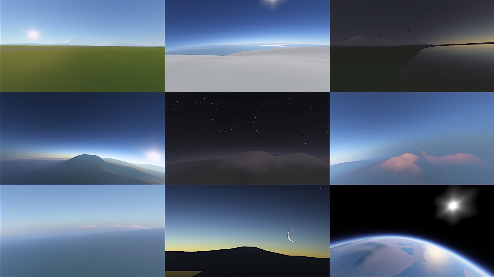 I want to emphasize that the above is rendered in software with nothing but Gouraud shading and vertex colors. This just as a reminder of how nice visuals can be driven by low tech. It ran also relatively fast (40 Hz in a resolution of 720p).
Moving it to the GPU
The article that I wrote for GPU Pro 3 describes the same algorithm as that which was running in my prototype, just with all code moved to the pixel shader, and wrapped in a ray-tracing framework (essentially “shadertoying” it). This approach is wasteful, a fact that was correctly pointed out in [12]. One can no longer benefit from triangle interpolation and cannot parallelize threads across sample points; instead the whole thing is a big loop per pixel.
Instead, atmospheric scattering should ideally be done with a kind of map-reduce operation: First calculate all sample points in parallel (the map part) and then collect the result along rays (the reduce part), similar to how my prototype worked. This could practically be done a compute shader, but I did not yet explore this idea further. The shadertoy that was linked in the beginning of this post also does the big-loop-in-the-pixel-shader approach, for lack of other practical alternatives.
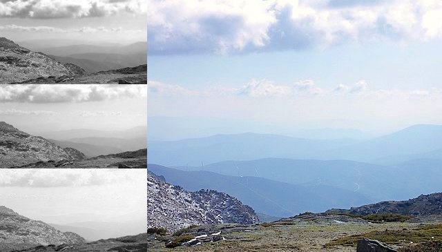
Aerial perspective — Photo taken from Wikipedia, CC-BY-SA Joaquim Alves Gaspar
Aerial perspective and spectral sampling
The visual impact of atmospheric scattering is called aerial perspective. It is not the same as fixed-function fog, but if we want to use that as an analogy, we would have to have a fog coordinate for each color channel. To illustrate, I have taken the photo from the top of the linked Wikipedia article and separated its color channels (see the insets above). It should be evident that the distant mountains are blue not because of some blue “fog color” (that would be white, in the limit of infinite distance), but rather because each channel has a different multiplier for the fog distance, the blue channel having the highest.
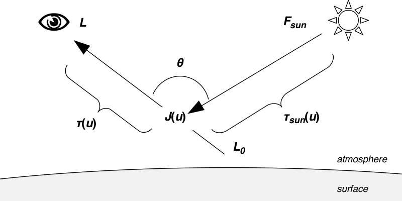
Formally, aerial perspective is a transformation of some original color  by a multiplicative operation, the transmittance
  , and an additive operation, the in-scatter
  (see also [1] for an introduction of these terms):
![\[L = T L_0 + I,\]](http://www.thetenthplanet.de/wordpress/wp-content/ql-cache/quicklatex.com-a2537be67492ed24c9a0d8cc18894844_l3.png "Rendered by QuickLaTeX.com")
where  , and are color vectors. In order to be universally valid and independent of the choice of color basis, the transmittance operator would have to be a tensor, as in
![\[L_\nu = T^\mu_\nu L_{0 \mu} + I_\nu,\]](http://www.thetenthplanet.de/wordpress/wp-content/ql-cache/quicklatex.com-56b45c32155cbdc29d89490b7b0f6327_l3.png "Rendered by QuickLaTeX.com")
where  ,
,  are spectral indices. If (and only if) is diagonal would it be appropriate to use the more familiar component-wise form
![\[L_\nu = T_\nu L_{0 \nu} + I_\nu.\]](http://www.thetenthplanet.de/wordpress/wp-content/ql-cache/quicklatex.com-9a273f83ce399a56da9d1e85729404e7_l3.png "Rendered by QuickLaTeX.com")
This opens up the question of color space. is trivially diagonal if the basis is simply the full spectrum (in infinite resolution). Otherwise the color basis must be carefully chosen to have properties of a chromatic adapation space. Following this clue I took the dominant wavelengths of the LMS cone responses as a starting point to settle for 615 nm for the red wavelength, 535 nm for the green wavelength and 445 nm for the blue wavelength. When these wavelengths are used as sample points together with a proper transform, the resulting colors are very accurate. I used the new CIE 2012 CMFs to calculate the transform from spectral samples to sRGB colors, as follows:
![\[M_{\text{615,535,445}\rightarrow\text{sRGB}} = \left( \begin{array}{d{4}d{4}d{4}} 1.6218 & -0.4493 & 0.0325 \\ -0.0374 & 1.0598 & -0.0742 \\ -0.0283 & -0.1119 & 1.0491 \end{array} \right) .\]](http://www.thetenthplanet.de/wordpress/wp-content/ql-cache/quicklatex.com-a2a3957443782f122707681b0951ba40_l3.png "Rendered by QuickLaTeX.com")
Side note: The matrix
from above looks red-heavy, because it contains an adaptation from white point E to D65. This was done so that the color components in this basis can be used as if they were spectral point samples. For example: the color of the sunlight spectrum, normalized to unit luminance, would be
in this basis, which corresponds very well to a point sampling of the smoothed sunlight spectrum at the wavelengths 615 nm, 535 nm and 445 nm. The transformation by
which has a correlated color temperature of 5778 K.
Geometry of the aerial perspective problem
The next problem is to find the numerical values for and . No solutions in closed form exist in the general case, so some sort of numerical integration needs to be performed.
- The transmittance is found as the antilogarithm of the optical depth
 , which in turn is found as the path integral of the extinction coefficient
  along lines of sight. The extinction coefficient is density dependent, so it varies as a function of the path coordinate
  .
. - The in-scatter is found similarly as the path integral of weighted with the source function
 attenuated by the cumulated optical depth
  along the path. The source function in turn – when only single scattering of sunlight is considered (also disregarding thermal emission) – equals incoming solar flux
  times a phase function
  times the single scattering albedo
  of the atmospheric material, and again attenuated by optical depth
  along the path towards the sun.
Note how the product  is always dimensionless.

It is evident that finding along (semi-infinite, treating the sun as infinitely distant) rays appears as a sub-problem of evaluating  . A real-time application must be able to do this in O(1) time. But again there is, in general, no simple solution for , since air density decreases exponentially with altitude, and the altitude above a spherical surface varies non-linearly along straight paths (and we have not even considered bending of rays at the horizon).
The Chapman function
As it is so often, problems in computer graphics have already been treated in physics literature. In this case, the optical depth along rays in a spherically symmetric, exponentially decreasing atmosphere was considered in the 1930’s by Sydney Chapman [2]. The eponymous Chapman function
![\[\operatorname{Ch}(x,\chi)\]](http://www.thetenthplanet.de/wordpress/wp-content/ql-cache/quicklatex.com-451c758b7653d4b995464c53550f37f5_l3.png "Rendered by QuickLaTeX.com")
is defined as relative optical depth along a semi-infinite ray having zenith angle  (read: greek letter chi), as seen by an observer at altitude
  (where is the radial distance to the sphere center expressed in multiples of the scale height). It is normalized to the zenith direction so
  for all . The following expression, distilled from a larger one in [3], can be taken as a
 virtually exact solution passable approximation (see Evgenii Golubev’s article over at Zero Radiance where he points out its flaws, and reference [13] for a more recent treatment):
![\begin{align*} \operatorname{Ch}&(x,\chi) = \frac{1}{2} \Bigg[ \cos(\chi) + \operatorname{erfcx} \left( \sqrt{ \frac{x \cos^2\chi}{2} } \right) \left( \frac{1}{x} + 2 - \cos^2\chi \right) \sqrt{\frac{\pi x}{2}} \Bigg] . \end{align*}](http://www.thetenthplanet.de/wordpress/wp-content/ql-cache/quicklatex.com-f96e5baba6d1b63fb4121361bc131909_l3.png "Rendered by QuickLaTeX.com")
Note how this expression contains  , the scaled complementary error function, which is a non-standard special function that one would need to implement on its own, so we’re back to square one. This is clearly not real-time friendly and needs to be simplified a lot.
An efficient approximation
My approximation was motivated by the fact that in the limit of a flat earth,  must approach the secant function. Therefore I looked for a low-order rational function of
  , such that it gives unity in the zenith direction and the special value
  in the horizontal direction. The expression for
  is already much simpler since
  vanishes, and I aggressively simplified it even more. The extension to zenith angles
  was then done by some trigonometric reasoning. The final result, as originally published, is

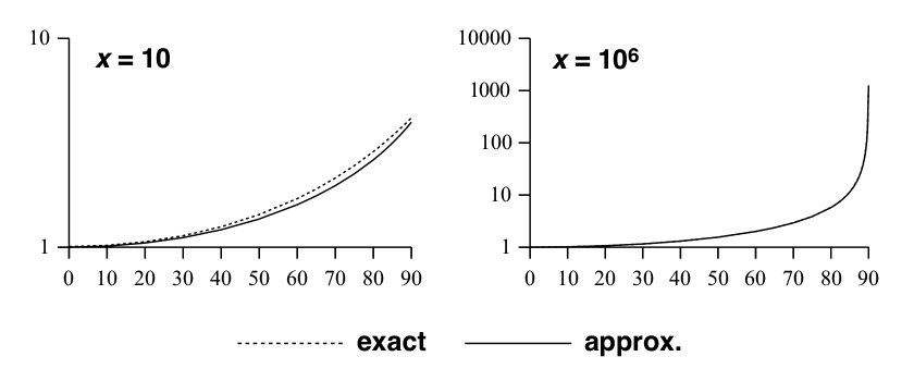
This is the main result. Note that the expensive case for when  only needs to be considered when looking downwards and the view is not already obscured by the terrain, which only applies to a small region below the horizon. A comparison between the exact and the approximate versions of
  is shown below:
Epilog: A literature review
At this point I want to stress how every real-time algorithm for atmospheric scattering must have an efficient way to evaluate , even when this function is not explicitly identified as such. Here is a small literature survey to illustrate that point:
| Author(s) | Type | Assumptions |  appears disguised in appears disguised in |
|---|---|---|---|
| Nishita et al. ’93 [4] | table | Parallel sunrays | Section 4.3.4 |
| Preetham et al. ’99 [5] | analytic | Earthbound observer | Appendix A.1 |
| Nielsen ’03 [6] | analytic | Hardcoded use case | Section 5.4.1 |
| O’Neil ’04 [7] | table | — | Sourcecode |
| O’Neil ’05 [8] | analytic | Constant  |
Section 4.2 |
| Schafhitzel et al. ’07 [9] | table | — | Section 4.1 |
| Bruneton, Neyret ’08 [10] | table | — | Section 4 as  |
| Schüler ’12 [11] | analytic | — | Listing 1 |
| Yusov ’14 [12] | analytic | — | Section 2.4.2 as  |
Outlook
This was the first post in a series. I originally didn’t plan to do a series but I decided to split when the word count went over 4000, especially with the source listings. The next post will explain an overflow-free implementation of the chapman function in shader code, how transmittances can be calculated along arbitrary rays and then guide through the procedure of integrating the atmospheric in-scatter along a viewing ray.
References
[1] Naty Hoffman and Arcot J Preetham (2002): “Rendering Outdoor Light Scattering in Real Time”
http://developer.amd.com/…
[2] Sydney Chapman (1931): “The absorption and dissociative or ionizing effect of monochromatic radiation in an atmosphere on a rotating earth.” Proceedings of the Physical Society 43:1, 26.
http://stacks.iop.org/…
[3] Miroslav Kocifaj (1996): “Optical Air Mass and Refraction in a Rayleigh Atmosphere.” Contributions of the Astronomical Observatory Skalnate Pleso 26:1, 23–30.
http://adsabs.harvard.edu/…
[4] Tomoyuki Nishita, Takao Sirai, Katsumi Tadamura and Eihachiro Nakamae (1993): “Display of the earth taking into account atmospheric scattering” Proceedings of the 20th annual conference on Computer graphics and interactive techniques, SIGGRAPH ’93, pp. 175–182.
http://doi.acm.org/…
[5] Arcot J Preetham, Peter Shirley and Brian Smits (1999): “A practical analytic model for daylight” Proceedings of the 26th annual conference on Computer graphics and interactive techniques, SIGGRAPH ’99, pp. 91–100
http://www2.cs.duke.edu/…
[6] Ralf Stockholm Nielsen (2003): “Real Time Rendering of Atmospheric Scattering Effects for Flight Simulators” Master’s thesis, Informatics and Mathematical Modelling, Technical University of Denmark
http://www2.imm.dtu.dk/…
[7] Sean O’Neil (2004): “Real-Time Atmospheric Scattering”
http://archive.gamedev.net/…
[8] Sean O’Neil (2005): “Accurate Atmospheric Scattering” GPU Gems 2, Pearson Addison Wesley Prof, pp. 253–268
http://developer.nvidia.com/…
[9] Tobias Schafhitzel, Martin Falk and Thomas Ertl (2007): “Real-Time Rendering of Planets with Atmospheres” Journal of WSCG 15, pp. 91–98
http://citeseerx.ist.psu.edu/…
[10] Éric Bruneton and Fabrice Neyret (2008): “Precomputed Atmospheric Scattering” Proceedings of the 19th Eurographics Symposium on Rendering, Comput. Graph. Forum 27:4, pp. 1079–1086
http://www-ljk.imag.fr/…
[11] Christian Schüler (2012): “An Approximation to the Chapman Grazing-Incidence Function for Atmospheric Scattering” GPU Pro 3, A K Peters, pp. 105–118.
http://books.google.de/…
[12] Egor Yusov (2014): “High Performance Outdoor Light Scattering using Epipolar Sampling” GPU Pro 5, A K Peters, pp. 101–126
http://books.google.de/…
[13] Dmytro Vasylyev (2021): “Accurate analytic approximation
for the Chapman grazing incidence function” Earth, Planets and Space 73:112
http://doi.org/10.1186/s40623-021–01435‑y
Pingback: Followup to GPU Pro3 Atmospheric Scattering—Part 1 via @KostasAAA | hanecci's blog : はねっちブログ
Hi, Thanks but the maths is above my head, whats the license of code in shadertoy? :)
Wow! Thanks, It’s beautiful!
Any chance to see the second part of this interesting series?
I would be really interested into hearing more about the color adaptation part. These are just a few questions that pop to mind:
* How is the matrix derived exactly? I guess the matrix is the result of multiplying the spectrum-to-srgb CMF matrix, and the color adaptation matrix. For the latter, did you use a Bradford or Von Kries transform to adapt from illuminant E to illuminant D65?
* What kind of improvements did you notice in practice by shifting color space?
* Did you notice better results by using CIE 2012 instead of the old 1931 CMF?
* In this workflow, the basis is essentially a spectrum intensity at the three different wavelengths. So, if I understand correctly, colors are not expressed in terms of “coordinates” within a gamut. Does this make it harder for artists to express colors in this way?
Hallo Sun,
I did a few experiments in order to settle down at exactly the wavelengths given. These experiments are as of yet unpublished (but your enquiry is just another hint for me that this needs to change :D). It turns out that there is only a very narrow range of wavelengths that can be chosen to make the transmittance operator approximately diagonal.
Once we have established that the transmittance operator is diagonal, there is no need for a Bradford transform or the like, we can just adapt the illuminant by componentwise multiplication, as if it was a transmittance trough a filter (that was the whole point of diagonalizing the operator!).
So the method to arrive at the matrix is
— use the sRGB CMFs sampled at 615, 535, 445 and stack them to a matrix ‘M*’, so that M* is the transform from sampled color space to sRGB
— get the components of illuminant E in sRGB
— multipliy illuminant E with the inverse of M*, giving ‘E*’
— scale columns of M* by component-weise by E*, giving M
The color space defined by M is just like any other color space having a gamut, a white point and its primaries.
One example where the custom color space really shows is looking at the turquoise shallow beachwater at a distance (through the atmosphere). The yellow sand is transmitted through the water, giving a (probably out of gamut) turqoise. Then the turquoise is transmitted through the atmosphere, which de-saturates and brings it into the sRGB gamut. But if we didn’t have the possibility to express the out of gamut color in the intermediate step, the end result would be much less lively.
@christian
Thank you, really interesting example you brought up.
One more thing I’m interested into is how this affects the data that are input to the simulation. Since sRGB is not used anymore, and calculations happen in M, then both luminance values (e.g. sun), as well as atmosphere parameters (e.g. rayleigh scattering, ozone absorption) should be expressed in a different space, is that correct?
If so, how would you derive this data to maintain correctness?
Yes, and they are!
For example, in the code of the linked shadertoy you can find these definitions, among others
const vec4  COL_AIRGLOW = 1.0154e-6 * vec4( .8670, 1.0899, .4332, 15. );

const vec4  COL_SUNLIGHT = vec4( 0.9420, 1.0269, 1.0242, .3 );

const vec3  COL_P43PHOSPHOR = vec3( 0.5335, 1.2621, 0.1874 );
etc…
So the 615/535/445 color space is just like any other old color space where you can convolve a spectrum to get the three color values (or analogously, convert the spectrum to sRGB and use the inverse matrix).
The ability to do spectral point-sampling with reasonable accuracy is just a bonus feature of this color space.
(Oh, and in the examples above, whenever there is a 4th component this is used for 1250 nm near-infrared, so you can ignore it for the sake of this argument.)
Pingback: 大気/散乱 – Site-Builder.wiki
Pingback: Caveat: Even NASA pictures may not be linear (or the wrong kind of linear) | The Tenth Planet
Nice article!
Will there be a part 2 eventually?